History of Computer

parts of computer

A computer is a general purpose device that can be programmed to carry out a set of arithmetic or logical operations automatically.Since a sequence of operations can be readily changed, the computer can solve more than one kind of problem.

Conventionally, a computer consists of at least one processing element, typically a central processing unit (CPU), and some form of memory.The processing element carries out arithmetic and logic operations, and a sequencing and control unit can change the order of operations in response to stored information. Peripheral devices allow information to be retrieved from an external source, and the result of operations saved and retrieved.

In World War II, mechanical analog computers were used for specialized military applications. During this time the first electronic digital computers were developed. Originally they were the size of a large room, consuming as much power as several hundred modern personal computers (PCs).^[1]

Modern computers based on integrated circuits are millions to billions of times more capable than the early machines, and occupy a fraction of the space.^[2] Simple computers are small enough to fit into mobile devices, and mobile computers can be powered by small batteries. Personal computers in their various forms are icons of the Information Age and are what most people think of as “computers.” However, the embedded computers found in many devices from MP3 players to fighter aircraft and from toys to industrial robots are the most numerous.

Etymology

The first use of the word “computer” was recorded in 1613 in a book called “The yong mans gleanings” by English writer Richard Braithwait I haue read the truest computer of Times, and the best Arithmetician that euer breathed, and he reduceth thy dayes into a short number. It referred to a person who carried out calculations, or computations, and the word continued with the same meaning until the middle of the 20th century. From the end of the 19th century the word began to take on its more familiar meaning, a machine that carries out computations

History

Rudimentary calculating devices first appeared in antiquity and mechanical calculating aids were invented in the 17th century. The first recorded use of the word “computer” is also from the 17th century, applied to human computers, people who performed calculations, often as employment. The first computer devices were conceived of in the 19th century, and only emerged in their modern form in the 1940s.

First general purpose computing device

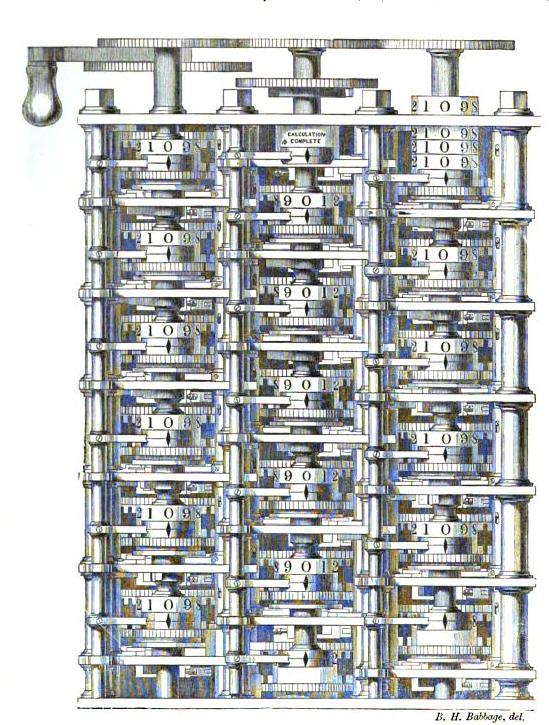
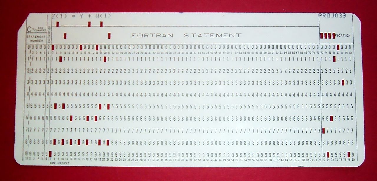
Charles Babbage, an English mechanical engineer and polymath, originated the concept of a programmable computer. Considered the “father of the computer“,^[4] he conceptualized and invented the first mechanical computer in the early 19th century. After working on his revolutionary difference engine, designed to aid in navigational calculations, in 1833 he realized that a much more general design, anAnalytical Engine, was possible. The input of programs and data was to be provided to the machine via punched cards, a method being used at the time to direct mechanical looms such as the Jacquard loom. For output, the machine would have a printer, a curve plotter and a bell. The machine would also be able to punch numbers onto cards to be read in later. The Engine incorporated an arithmetic logic unit, control flow in the form of conditional branching and loops, and integrated memory, making it the first design for a general-purpose computer that could be described in modern terms as Turing-complete.^[5][6]

The machine was about a century ahead of its time. All the parts for his machine had to be made by hand – this was a major problem for a device with thousands of parts. Eventually, the project was dissolved with the decision of the British Government to cease funding. Babbage’s failure to complete the analytical engine can be chiefly attributed to difficulties not only of politics and financing, but also to his desire to develop an increasingly sophisticated computer and to move ahead faster than anyone else could follow. Nevertheless his son, Henry Babbage, completed a simplified version of the analytical engine’s computing unit (the mill) in 1888. He gave a successful demonstration of its use in computing tables in 1906.

Early analog computers

During the first half of the 20th century, many scientific computing needs were met by increasingly sophisticated analog computers, which used a direct mechanical or electrical model of the problem as a basis for computation. However, these were not programmable and generally lacked the versatility and accuracy of modern digital computers.^[7]

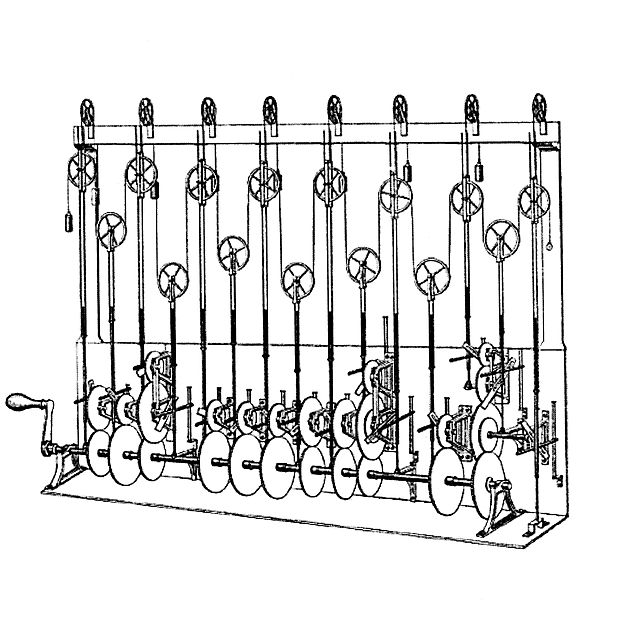
The first modern analog computer was a tide-predicting machine, invented by Sir William Thomson in 1872. The differential analyser, a mechanical analog computer designed to solve differential equations by integration using wheel-and-disc mechanisms, was conceptualized in 1876 by James Thomson, the brother of the more famous Lord Kelvin.^[8]

The art of mechanical analog computing reached its zenith with the differential analyzer, built by H. L. Hazen and Vannevar Bush at MIT starting in 1927. This built on the mechanical integrators of James Thomson and the torque amplifiers invented by H. W. Nieman. A dozen of these devices were built before their obsolescence became obvious.

The first electromechanical computer

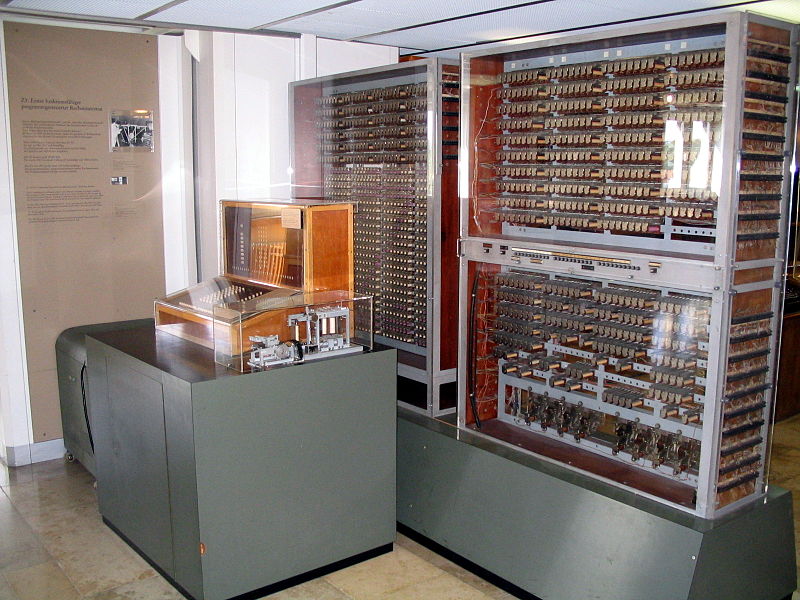
Early digital computers were electromechanical; electric switches drove mechanical relays to perform the calculation. These devices had a low operating speed and were eventually superseded by much faster all-electric computers, originally using vacuum tubes. The Z2, created by German engineer Konrad Zuse in 1939, was one of the earliest examples of an electromechanical relay computer.^[11]

In 1941, Zuse followed his earlier machine up with the Z3, the world’s first working electromechanical programmable, fully automatic digital computer.^[12][13] The Z3 was built with 2000 relays, implementing a 22 bit word length that operated at a clock frequency of about 5–10 Hz.^[14]Program code and data were stored on punched film. It was quite similar to modern machines in some respects, pioneering numerous advances such as floating point numbers. Replacement of the hard-to-implement decimal system (used in Charles Babbage‘s earlier design) by the simpler binary system meant that Zuse’s machines were easier to build and potentially more reliable, given the technologies available at that time.^[15] The Z3 was probably a complete Turing machine.

The introduction of electronic programmable computers with vacuum tubes

Purely electronic circuit elements soon replaced their mechanical and electromechanical equivalents, at the same time that digital calculation replaced analog. The engineer Tommy Flowers, working at the Post Office Research Station in London in the 1930s, began to explore the possible use of electronics for the telephone exchange. Experimental equipment that he built in 1934 went into operation 5 years later, converting a portion of the telephone exchange network into an electronic data processing system, using thousands of vacuum tubes.^[7] In the US, John Vincent Atanasoff and Clifford E. Berry of Iowa State University developed and tested the Atanasoff–Berry Computer (ABC) in 1942,^[16] the first “automatic electronic digital computer”.^[17] This design was also all-electronic and used about 300 vacuum tubes, with capacitors fixed in a mechanically rotating drum for memory.

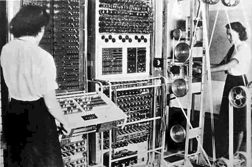
During World War II, the British at Bletchley Park achieved a number of successes at breaking encrypted German military communications. The German encryption machine, Enigma, was first attacked with the help of the electro-mechanical bombes. To crack the more sophisticated German Lorenz SZ 40/42 machine, used for high-level Army communications, Max Newman and his colleagues commissioned Flowers to build the Colossus.He spent eleven months from early February 1943 designing and building the first Colossus. After a functional test in December 1943, Colossus was shipped to Bletchley Park, where it was delivered on 18 January 1944 and attacked its first message on 5 February.

Colossus was the world’s first electronic digital programmable computer. It used a large number of valves (vacuum tubes). It had paper-tape input and was capable of being configured to perform a variety of boolean logical operations on its data, but it was not Turing-complete. Nine Mk II Colossi were built (The Mk I was converted to a Mk II making ten machines in total). Colossus Mark I contained 1500 thermionic valves (tubes), but Mark II with 2400 valves, was both 5 times faster and simpler to operate than Mark 1, greatly speeding the decoding process.

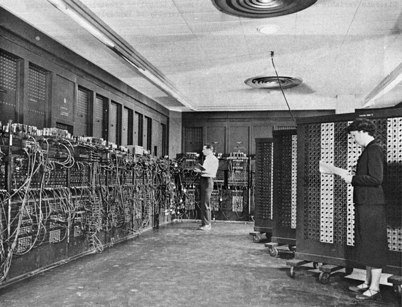
The US-built ENIAC^[23] (Electronic Numerical Integrator and Computer) was the first electronic programmable computer built in the US. Although the ENIAC was similar to the Colossus it was much faster and more flexible. It was unambiguously a Turing-complete device and could compute any problem that would fit into its memory. Like the Colossus, a “program” on the ENIAC was defined by the states of its patch cables and switches, a far cry from the stored program electronic machines that came later. Once a program was written, it had to be mechanically set into the machine with manual resetting of plugs and switches.

It combined the high speed of electronics with the ability to be programmed for many complex problems. It could add or subtract 5000 times a second, a thousand times faster than any other machine. It also had modules to multiply, divide, and square root. High speed memory was limited to 20 words (about 80 bytes). Built under the direction of John Mauchly and J. Presper Eckert at the University of Pennsylvania, ENIAC’s development and construction lasted from 1943 to full operation at the end of 1945. The machine was huge, weighing 30 tons, using 200 kilowatts of electric power and contained over 18,000 vacuum tubes, 1,500 relays, and hundreds of thousands of resistors, capacitors, and inductors

Stored program computers eliminate the need for re-wiring

Early computing machines had fixed programs. Changing its function required the re-wiring and re-structuring of the machine. With the proposal of the stored-program computer this changed. A stored-program computer includes by design an instruction set and can store in memory a set of instructions (a program) that details the computation. The theoretical basis for the stored-program computer was laid by Alan Turing in his 1936 paper. In 1945 Turing joined the National Physical Laboratory and began work on developing an electronic stored-program digital computer. His 1945 report ‘Proposed Electronic Calculator’ was the first specification for such a device.John von Neumann at the University of Pennsylvania, also circulated his First Draft of a Report on the EDVAC in 1945.

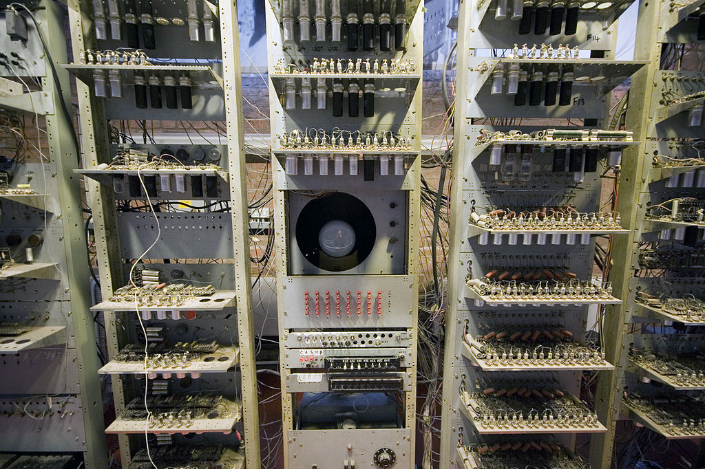
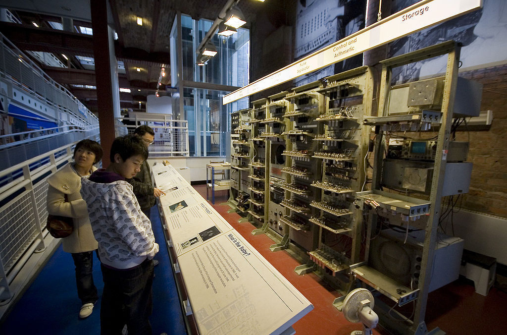
The Manchester Small-Scale Experimental Machine, nicknamed Baby, was the world’s first stored-program computer. It was built at the Victoria University of Manchester by Frederic C. Williams, Tom Kilburn and Geoff Tootill, and ran its first program on 21 June 1948. It was designed as a testbedfor the Williams tube the first random-access digital storage device. Although the computer was considered “small and primitive” by the standards of its time, it was the first working machine to

contain all of the elements essential to a modern electronic computer. As soon as the SSEM had demonstrated the feasibility of its design, a project was initiated at the university to develop it into a more usable computer, the Manchester Mark 1.

The Mark 1 in turn quickly became the prototype for the Ferranti Mark 1, the world’s first commercially available general-purpose computer. Built by Ferranti, it was delivered to the University of Manchester in February 1951. At least seven of these later machines were delivered between 1953 and 1957, one of them to Shell labs in Amsterdam. In October 1947, the directors of British catering company J. Lyons & Company decided to take an active role in promoting the commercial development of computers. The LEO I computer became operational in April 1951  and ran the world’s first regular routine office computer job.

Transistor replace vacuum tubes in computer

The bipolar transistor was invented in 1947. From 1955 onwards transistors replaced vacuum tubes in computer designs, giving rise to the “second generation” of computers. Compared to vacuum tubes, transistors have many advantages: they are smaller, and require less power than vacuum tubes, so give off less heat. Silicon junction transistors were much more reliable than vacuum tubes and had longer, indefinite, service life. Transistorized computers could contain tens of thousands of binary logic circuits in a relatively compact space.

At the University of Manchester, a team under the leadership of Tom Kilburn designed and built a machine using the newly developedtransistors instead of valves.Their first transistorised computer and the first in the world, was operational by 1953, and a second version was completed there in April 1955. However, the machine did make use of valves to generate its 125 kHz clock waveforms and in the circuitry to read and write on its magnetic drum memory, so it was not the first completely transistorized computer. That distinction goes to the Harwell CADET of 1955, built by the electronics division of the Atomic Energy Research Establishment at Harwell.

Integrated circuits replace transistors

The next great advance in computing power came with the advent of the integrated circuit. The idea of the integrated circuit was first conceived by a radar scientist working for theRoyal Radar Establishment of the Ministry of Defence, Geoffrey W.A. Dummer. Dummer presented the first public description of an integrated circuit at the Symposium on Progress in Quality Electronic Components in Washington, D.C. on 7 May 1952.
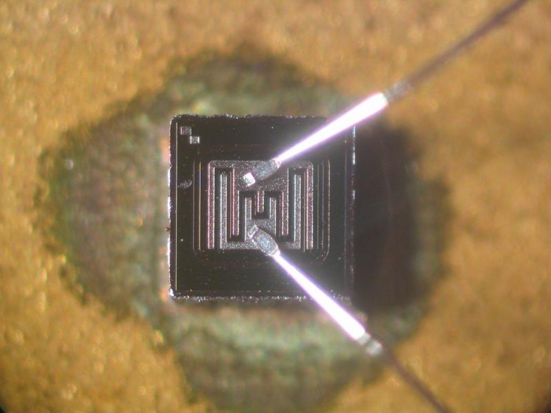
The first practical ICs were invented by Jack Kilby at Texas Instruments and Robert Noyce at Fairchild Semiconductor. Kilby recorded his initial ideas concerning the integrated circuit in July 1958, successfully demonstrating the first working integrated example on 12 September 1958. In his patent application of 6 February 1959, Kilby described his new device as “a body of semiconductor material … wherein all the components of the electronic circuit are completely integrated.” Noyce also came up with his own idea of an integrated circuit half a year later than Kilby. His chip solved many practical problems that Kilby’s had not. Produced at Fairchild Semiconductor, it was made of silicon, whereas Kilby’s chip was made of germanium.

This new development heralded an explosion in the commercial and personal use of computers and led to the invention of the microprocessor. While the subject of exactly which device was the first microprocessor is contentious, partly due to lack of agreement on the exact definition of the term “microprocessor”, it is largely undisputed that the first single-chip microprocessor was the Intel 4004, designed and realized by Ted Hoff, Federico Faggin, and Stanley Mazor at Intel.

Mobility and the growth of smartphone computers

With the continued miniaturization of computing resources, and advancements in portable battery life, portable computers grew in popularity in the 1990s. The same developments that spurred the growth of laptop computers and other portable computers allowed manufacturers to integrate computing resources into cellular phones. These so-called smartphones run on a variety of operating systems and are rapidly becoming the dominant computing device on the market, with manufacturers reporting having shipped an estimated 237 million devices in 2Q 2013.

 Programs

The defining feature of modern computers which distinguishes them from all other machines is that they can be programmed. That is to say that some type of instructions (theprogram) can be given to the computer, and it will process them. Modern computers based on the von Neumann architecture often have machine code in the form of an imperative programming language.

In practical terms, a computer program may be just a few instructions or extend to many millions of instructions, as do the programs for word processors and web browsers for example. A typical modern computer can execute billions of instructions per second (gigaflops) and rarely makes a mistake over many years of operation. Large computer programs consisting of several million instructions may take teams of programmers years to write, and due to the complexity of the task almost certainly contain errors.

Stored Program architecture

This section applies to most common RAM machine-based computers.

In most cases, computer instructions are simple: add one number to another, move some data from one location to another, send a message to some external device, etc. These instructions are read from the computer’s memory and are generally carried out (executed) in the order they were given. However, there are usually specialized instructions to tell the computer to jump ahead or backwards to some other place in the program and to carry on executing from there. These are called “jump” instructions (or branches). Furthermore, jump instructions may be made to happen conditionally so that different sequences of instructions may be used depending on the result of some previous calculation or some external event. Many computers directly support subroutines by providing a type of jump that “remembers” the location it jumped from and another instruction to return to the instruction following that jump instruction.

Program execution might be likened to reading a book. While a person will normally read each word and line in sequence, they may at times jump back to an earlier place in the text or skip sections that are not of interest. Similarly, a computer may sometimes go back and repeat the instructions in some section of the program over and over again until some internal condition is met. This is called the flow of control within the program and it is what allows the computer to perform tasks repeatedly without human intervention.

Comparatively, a person using a pocket calculator can perform a basic arithmetic operation such as adding two numbers with just a few button presses. But to add together all of the numbers from 1 to 1,000 would take thousands of button presses and a lot of time, with a near certainty of making a mistake. On the other hand, a computer may be programmed to do this with just a few simple instructions. For example:

[message_box title="" color="yellow"]   
  mov No. 0, sum     ; set sum to 0
      mov No. 1, num     ; set num to 1
loop: add num, sum    ; add num to sum
      add No. 1, num     ; add 1 to num
      cmp num, #1000  ; compare num to 1000
      ble loop        ; if num <= 1000, go back to 'loop'
      halt            ; end of program. stop running 
[/message_box]
Once told to run this program, the computer will perform the repetitive addition task without further human intervention. It will almost never make a mistake and a modern PC can complete the task in about a millionth of a second.

Machine code

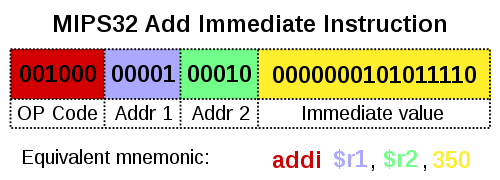
In most computers, individual instructions are stored as machine code with each instruction being given a unique number (its operation code or opcode for short). The command to add two numbers together would have one opcode; the command to multiply them would have a different opcode, and so on. The simplest computers are able to perform any of a handful of different instructions; the more complex computers have several hundred to choose from, each with a unique numerical code. Since the computer’s memory is able to store numbers, it can also store the instruction codes. This leads to the important fact that entire programs (which are just lists of these instructions) can be represented as lists of numbers and can themselves be manipulated inside the computer in the same way as numeric data. The fundamental concept of storing programs in the computer’s memory alongside the data they operate on is the crux of the von Neumann, or stored program^{[citation needed]}, architecture. In some cases, a computer might store some or all of its program in memory that is kept separate from the data it operates on. This is called the Harvard architecture after the Harvard Mark I computer. Modern von Neumann computers display some traits of the Harvard architecture in their designs, such as in CPU caches.

While it is possible to write computer programs as long lists of numbers (machine language) and while this technique was used with many early computers,^[45] it is extremely tedious and potentially error-prone to do so in practice, especially for complicated programs. Instead, each basic instruction can be given a short name that is indicative of its function and easy to remember – a mnemonic such as ADD, SUB, MULT or JUMP. These mnemonics are collectively known as a computer’s assembly language. Converting programs written in assembly language into something the computer can actually understand (machine language) is usually done by a computer program called an assembler.

Programming language

Programming languages provide various ways of specifying programs for computers to run. Unlike natural languages, programming languages are designed to permit no ambiguity and to be concise. They are purely written languages and are often difficult to read aloud. They are generally either translated into machine code by a compiler or an assembler before being run, or translated directly at run time by an interpreter. Sometimes programs are executed by a hybrid method of the two techniques.

Low-level languages

Machine languages and the assembly languages that represent them (collectively termed low-level programming languages) tend to be unique to a particular type of computer. For instance, an ARM architecture computer (such as may be found in a PDA or a hand-held videogame) cannot understand the machine language of an Intel Pentium or the AMD Athlon 64 computer that might be in a PC.

Higher-level languages

Though considerably easier than in machine language, writing long programs in assembly language is often difficult and is also error prone. Therefore, most practical programs are written in more abstract high-level programming languages that are able to express the needs of the programmer more conveniently (and thereby help reduce programmer error). High level languages are usually “compiled” into machine language (or sometimes into assembly language and then into machine language) using another computer program called a compiler.^[47] High level languages are less related to the workings of the target computer than assembly language, and more related to the language and structure of the problem(s) to be solved by the final program. It is therefore often possible to use different compilers to translate the same high level language program into the machine language of many different types of computer. This is part of the means by which software like video games may be made available for different computer architectures such as personal computers and various video game consoles.

Components

A general purpose computer has four main components: the arithmetic logic unit (ALU), the control unit, the memory, and the input and output devices (collectively termed I/O). These parts are interconnected by buses, often made of groups of wires.

Inside each of these parts are thousands to trillions of small electrical circuits which can be turned off or on by means of an electronic switch. Each circuit represents a bit (binary digit) of information so that when the circuit is on it represents a “1”, and when off it represents a “0” (in positive logic representation). The circuits are arranged in logic gates so that one or more of the circuits may control the state of one or more of the other circuits.

The control unit, ALU, registers, and basic I/O (and often other hardware closely linked with these) are collectively known as a central processing unit (CPU). Early CPUs were composed of many separate components but since the mid-1970s CPUs have typically been constructed on a single integrated circuit called a microprocessor.

Control unit

The control unit (often called a control system or central controller) manages the computer’s various components; it reads and interprets (decodes) the program instructions, transforming them into a series of control signals which activate other parts of the computer.^[50] Control systems in advanced computers may change the order of some instructions so as to improve performance.

A key component common to all CPUs is the program counter, a special memory cell (a register) that keeps track of which location in memory the next instruction is to be read from.^[51]

The control system’s function is as follows—note that this is a simplified description, and some of these steps may be performed concurrently or in a different order depending on the type of CPU:

1. Read the code for the next instruction from the cell indicated by the program counter.
2. Decode the numerical code for the instruction into a set of commands or signals for each of the other systems.
3. Increment the program counter so it points to the next instruction.
4. Read whatever data the instruction requires from cells in memory (or perhaps from an input device). The location of this required data is typically stored within the instruction code.
5. Provide the necessary data to an ALU or register.
6. If the instruction requires an ALU or specialized hardware to complete, instruct the hardware to perform the requested operation.
7. Write the result from the ALU back to a memory location or to a register or perhaps an output device.
8. Jump back to step (1).

Since the program counter is (conceptually) just another set of memory cells, it can be changed by calculations done in the ALU. Adding 100 to the program counter would cause the next instruction to be read from a place 100 locations further down the program. Instructions that modify the program counter are often known as “jumps” and allow for loops (instructions that are repeated by the computer) and often conditional instruction execution (both examples of control flow).

The sequence of operations that the control unit goes through to process an instruction is in itself like a short computer program, and indeed, in some more complex CPU designs, there is another yet smaller computer called a microsequencer, which runs a microcode program that causes all of these events to happen.

Arithmetic logic unit (ALU)

The ALU is capable of performing two classes of operations: arithmetic and logic.^[52]

The set of arithmetic operations that a particular ALU supports may be limited to addition and subtraction, or might include multiplication, division, trigonometry functions such as sine, cosine, etc., and square roots. Some can only operate on whole numbers (integers) whilst others use floating point to represent real numbers, albeit with limited precision. However, any computer that is capable of performing just the simplest operations can be programmed to break down the more complex operations into simple steps that it can perform. Therefore, any computer can be programmed to perform any arithmetic operation—although it will take more time to do so if its ALU does not directly support the operation. An ALU may also compare numbers and return boolean truth values (true or false) depending on whether one is equal to, greater than or less than the other (“is 64 greater than 65?”).

Logic operations involve Boolean logic: AND, OR, XOR and NOT. These can be useful for creating complicated conditional statements and processing boolean logic.

Superscalar computers may contain multiple ALUs, allowing them to process several instructions simultaneously.^[53] Graphics processors and computers with SIMD and MIMDfeatures often contain ALUs that can perform arithmetic on vectors and matrices.

Memory

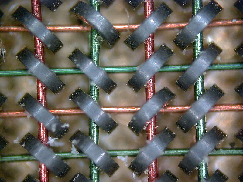
A computer’s memory can be viewed as a list of cells into which numbers can be placed or read. Each cell has a numbered “address” and can store a single number. The computer can be instructed to “put the number 123 into the cell numbered 1357” or to “add the number that is in cell 1357 to the number that is in cell 2468 and put the answer into cell 1595.” The information stored in memory may represent practically anything. Letters, numbers, even computer instructions can be placed into memory with equal ease. Since the CPU does not differentiate between different types of information, it is the software’s responsibility to give significance to what the memory sees as nothing but a series of numbers.

In almost all modern computers, each memory cell is set up to store binary numbers in groups of eight bits (called a byte). Each byte is able to represent 256 different numbers (2^8 = 256); either from 0 to 255 or −128 to +127. To store larger numbers, several consecutive bytes may be used (typically, two, four or eight). When negative numbers are required, they are usually stored in two’s complement notation. Other arrangements are possible, but are usually not seen outside of specialized applications or historical contexts. A computer can store any kind of information in memory if it can be represented numerically. Modern computers have billions or even trillions of bytes of memory.

The CPU contains a special set of memory cells called registers that can be read and written to much more rapidly than the main memory area. There are typically between two and one hundred registers depending on the type of CPU. Registers are used for the most frequently needed data items to avoid having to access main memory every time data is needed. As data is constantly being worked on, reducing the need to access main memory (which is often slow compared to the ALU and control units) greatly increases the computer’s speed.

Computer main memory comes in two principal varieties: random-access memory or RAM and read-only memory or ROM. RAM can be read and written to anytime the CPU commands it, but ROM is preloaded with data and software that never changes, therefore the CPU can only read from it. ROM is typically used to store the computer’s initial start-up instructions. In general, the contents of RAM are erased when the power to the computer is turned off, but ROM retains its data indefinitely. In a PC, the ROM contains a specialized program called the BIOS that orchestrates loading the computer’s operating system from the hard disk drive into RAM whenever the computer is turned on or reset. In embedded computers, which frequently do not have disk drives, all of the required software may be stored in ROM. Software stored in ROM is often called firmware, because it is notionally more like hardware than software. Flash memory blurs the distinction between ROM and RAM, as it retains its data when turned off but is also rewritable. It is typically much slower than conventional ROM and RAM however, so its use is restricted to applications where high speed is unnecessary.^[54]

In more sophisticated computers there may be one or more RAM cache memories, which are slower than registers but faster than main memory. Generally computers with this sort of cache are designed to move frequently needed data into the cache automatically, often without the need for any intervention on the programmer’s part.

Input/output  (I/O)

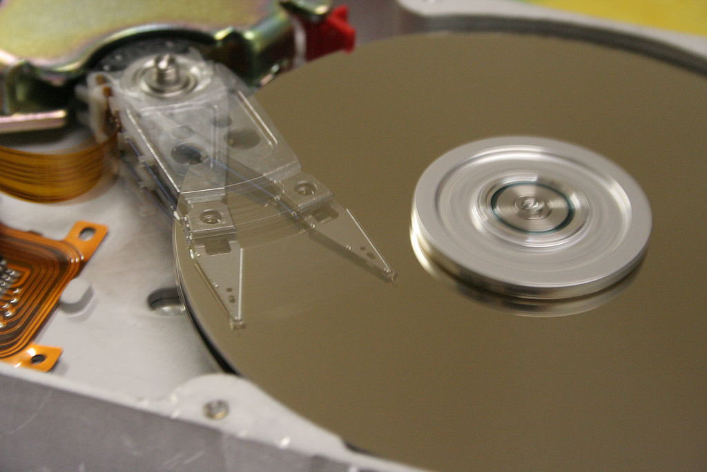
I/O is the means by which a computer exchanges information with the outside world.^[55] Devices that provide input or output to the computer are called peripherals.^[56] On a typical personal computer, peripherals include input devices like the keyboard and mouse, and output devices such as the display and printer. Hard disk drives, floppy disk drives and optical disc drives serve as both input and output devices. Computer networking is another form of I/O.

I/O devices are often complex computers in their own right, with their own CPU and memory. A graphics processing unit might contain fifty or more tiny computers that perform the calculations necessary to display 3D graphics.^{[citation needed]} Modern desktop computers contain many smaller computers that assist the main CPU in performing I/O.

Multitasking

While a computer may be viewed as running one gigantic program stored in its main memory, in some systems it is necessary to give the appearance of running several programs simultaneously. This is achieved by multitasking i.e. having the computer switch rapidly between running each program in turn.^[57]

One means by which this is done is with a special signal called an interrupt, which can periodically cause the computer to stop executing instructions where it was and do something else instead. By remembering where it was executing prior to the interrupt, the computer can return to that task later. If several programs are running “at the same time,” then the interrupt generator might be causing several hundred interrupts per second, causing a program switch each time. Since modern computers typically execute instructions several orders of magnitude faster than human perception, it may appear that many programs are running at the same time even though only one is ever executing in any given instant. This method of multitasking is sometimes termed “time-sharing” since each program is allocated a “slice” of time in turn.^[58]

Before the era of cheap computers, the principal use for multitasking was to allow many people to share the same computer.

Seemingly, multitasking would cause a computer that is switching between several programs to run more slowly, in direct proportion to the number of programs it is running, but most programs spend much of their time waiting for slow input/output devices to complete their tasks. If a program is waiting for the user to click on the mouse or press a key on the keyboard, then it will not take a “time slice” until the event it is waiting for has occurred. This frees up time for other programs to execute so that many programs may be run simultaneously without unacceptable speed loss.

Multiprocessing

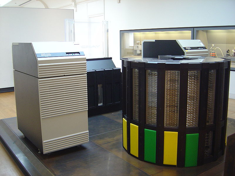
Some computers are designed to distribute their work across several CPUs in a multiprocessing configuration, a technique once employed only in large and powerful machines such as supercomputers, mainframe computers and servers. Multiprocessor and multi-core (multiple CPUs on a single integrated circuit) personal and laptop computers are now widely available, and are being increasingly used in lower-end markets as a result.

Supercomputers in particular often have highly unique architectures that differ significantly from the basic stored-program architecture and from general purpose computers.^[59] They often feature thousands of CPUs, customized high-speed interconnects, and specialized computing hardware. Such designs tend to be useful only for specialized tasks due to the large scale of program organization required to successfully utilize most of the available resources at once. Supercomputers usually see usage in large-scale simulation, graphics rendering, and cryptography applications, as well as with other so-called “embarrassingly parallel” tasks.

Networking and Internet

Computers have been used to coordinate information between multiple locations since the 1950s. The U.S. military’s SAGE system was the first large-scale example of such a system, which led to a number of special-purpose commercial systems such as Sabre.^[60]

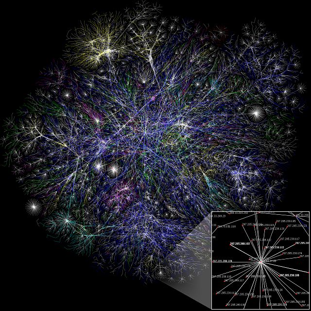
In the 1970s, computer engineers at research institutions throughout the United States began to link their computers together using telecommunications technology. The effort was funded by ARPA (now DARPA), and the computer network that resulted was called theARPANET.^[61] The technologies that made the Arpanet possible spread and evolved.

In time, the network spread beyond academic and military institutions and became known as the Internet. The emergence of networking involved a redefinition of the nature and boundaries of the computer. Computer operating systems and applications were modified to include the ability to define and access the resources of other computers on the network, such as peripheral devices, stored information, and the like, as extensions of the resources of an individual computer. Initially these facilities were available primarily to people working in high-tech environments, but in the 1990s the spread of applications like e-mail and the World Wide Web, combined with the development of cheap, fast networking technologies like Ethernet and ADSL saw computer networking become almost ubiquitous. In fact, the number of computers that are networked is growing phenomenally. A very large proportion of personal computers regularly connect to the Internet to communicate and receive information. “Wireless” networking, often utilizing mobile phone networks, has meant networking is becoming increasingly ubiquitous even in mobile computing environments.